How to read a spectrum analyzer, pre vs post
An analyzer only tells the truth if you know its FFT size, tilt, and smoothing. What each setting hides, and how to hunt a resonance with the display.
The spectrum analyzer is the most watched and least understood display in a session. Everyone leaves one open. Very few people could say what their analyzer's FFT size is, what slope it draws pink noise at, or whether the trace they are staring at is smoothed enough to hide the exact problem they opened it to find.
This article walks the mechanism: what one frame of the display actually measures, what each setting trades away, why pre and post taps answer different questions, and how to run a resonance hunt where the analyzer helps instead of decorates.
What one frame of the display actually is
An FFT analyzer grabs a block of samples, N of them, and reports how much energy sits in N/2 evenly spaced frequency bins from zero up to half the sample rate. That is the whole machine. A 4096-point FFT at 48 kHz gives you bins spaced about 11.7 Hz apart.
The catch is that the bins are spaced linearly and the display axis, like your hearing, is logarithmic. At 11.7 Hz spacing, the octave from 10 kHz to 20 kHz contains roughly 850 bins. The octave from 40 to 80 Hz contains three or four. So the top of the display is squeezing hundreds of bins into a few pixels, while the bottom is stretching a handful of bins across the widest, most contested region of the mix. Whatever precision an analyzer has, it has the least of it exactly where bass decisions get made.
FFT size: resolution against speed
A bigger FFT narrows the bins. It also lengthens the block: 4096 samples at 48 kHz is about 85 milliseconds of audio, so each frame of the display describes almost a tenth of a second, and the trace responds sluggishly to fast material. A small FFT is the opposite. A 1024-point analysis updates quickly and feels snappy, but its bins are about 47 Hz wide, which means everything below 100 Hz lands in two or three bins. It physically cannot tell you whether the problem is at 55 Hz or 80 Hz. It does not have the number.
The practical rule: use a large FFT when you are inspecting low end, and never trust the bottom octave of a fast, small-FFT display. The wobble you see there is bin granularity, not the bass.
Tilt: why flat does not look flat
Music carries roughly equal energy per octave, not per hertz. Since each octave upward spans twice as many hertz, the energy in any one bin falls as frequency rises. Draw a well-balanced mix on a raw per-bin analyzer and it slopes downward at about 3 dB per octave.
To compensate, analyzers apply a tilt, commonly 3 to 4.5 dB per octave, so balanced program draws approximately level. This is a display convention, not a measurement, and different tools pick different slopes. If you do not know your analyzer's tilt, you do not know what "flat" on it means, and traces from two plugins with different slopes are not comparable. White noise, which has equal energy per hertz and sounds piercingly bright, is what actually draws flat on an untilted display. That alone should end the habit of mixing toward a level line.
Averaging and smoothing hide different things
These two settings get conflated because both make the trace calmer. They operate on different axes and they hide different information.
Averaging works across time: each drawn frame blends the last several FFT frames. Long averaging gives you a steady trace that reads like the tonal fingerprint of the material, which is exactly what you want when judging overall balance, and exactly what erases transients. A snare's crack does not survive the blend; only its sustain does.
Smoothing works across frequency: each drawn point blends neighboring bins, usually specified in fractions of an octave like 1/3 or 1/6. It produces the smooth, publishable kind of curve. It also spreads any narrow feature across the smoothing window. A resonance one third of an octave wide, run through 1/3-octave smoothing, gets its energy shared out with its neighbors and can drop enough decibels to disappear into the trace entirely.
That is the trap worth naming. A ringing resonance, the boxy hum in a room mic, the note a snare shell will not let go of, is precisely a narrow, steady spike. Narrow and steady is the one combination that frequency smoothing is built to erase and that time averaging is built to reveal. So the hunting configuration is the reverse of the pretty one: smoothing off or minimal, averaging slow, or a peak-hold trace. Broadband content averages toward its mean and the parked spike accumulates until it stands up out of the floor.
Pre and post answer different questions
An analyzer inside an EQ can tap the signal before your curve or after it. The distinction shapes the whole workflow.
| Tap | What it shows | What it is for |
|---|---|---|
| Pre | The source, untouched by your bands | Diagnosis: finding the problem, keeping a fixed reference |
| Post | The source through the summed curve | Verification: confirming the fix landed where you aimed |
The failure mode is diagnosing from post. Every band you move reshapes the trace you are reading, so the target drifts with every adjustment and you end up chasing your own EQ. Diagnose on pre, where the spike holds still no matter what you do. Then flip to post to confirm the cut is centered on the spike and deep enough, and that the rest of the curve did not tilt something you did not intend.
The resonance hunt, step by step
With the display configured honestly, the hunt itself is short. Listen first and form a guess: boxy suggests low mids, honky suggests upper mids, a ring on a drum is usually a specific note. Then read the pre trace, unsmoothed, slow averaged, and look for a spike that stays parked while the music moves around it. Drop a narrow bell there, solo the band so you hear only what it passes, and tighten the bandwidth until the ring isolates from the material around it. Flip the boost to a cut and take only as much as it needs to stop poking out.
- Notes are peaks too. A spike that moves with the performance is the music. A resonance stays at one frequency across different notes and sections. Watch the trace over time before you commit to cutting anything.
- Check the multiples. Rings and room modes rarely come alone. If the fundamental parks at one frequency, look for smaller spikes near two and three times it before declaring the job done.
- Solo exaggerates. Band solo is for finding the frequency, not for choosing the depth. A ring that sounds offensive in isolation may need only a few dB of cut in context. Set the depth with the solo off.
- A boosted sweep biases you. Sweeping a 12 dB narrow boost makes every frequency sound like a problem. If you sweep, sweep to locate, then reassess at unity before cutting.
A worked example
Here is the loop as it runs in Bevel EQ, which draws its real-time analyzer directly under the summed curve, drawing the pre and post traces at the same time. Say a room mic has a boxy ring. Let it run while the section plays: a spike holds its position through the chord changes, so it is the room, not the writing. Double-click the curve on it and engage that band's solo to hear exactly what the band passes; tighten Q until the ring sits alone. Because frequency, gain and Q are typeable, you can set the center exactly where the spike reads. Flip the gain negative and kill the solo. Now the two traces do the work for you: the post trace should show the spike gone while the pre trace still shows it, so you can see the cut and the original in one glance instead of toggling between them. Save the result as an A/B state and toggle against the untouched state to confirm you fixed the ring rather than dulled the room. The analyzer runs on the UI thread, not in the audio path, so leaving it open costs the session nothing.